Intro to Control Theory & Laplace Transform

Course Overview

The aims of this module are to:

• Introduce feedback systems and the concepts of block diagrams and transfer functions and different types of controllers
• Introduce the concept of stability and performance criteria of feedback systems
• Explain the concept of root locus and its application to classical control design
• Introduce frequency response and Bode diagrams-based analysis and design techniques

Having successfully completed the module, you will be able to:

• determine the step transient response of a system
• determine the frequency response of a system

---

Types of Control system

Open loop control

• No feedback, only operator input

Closed loop control

• Feedback control system automates optimization

---

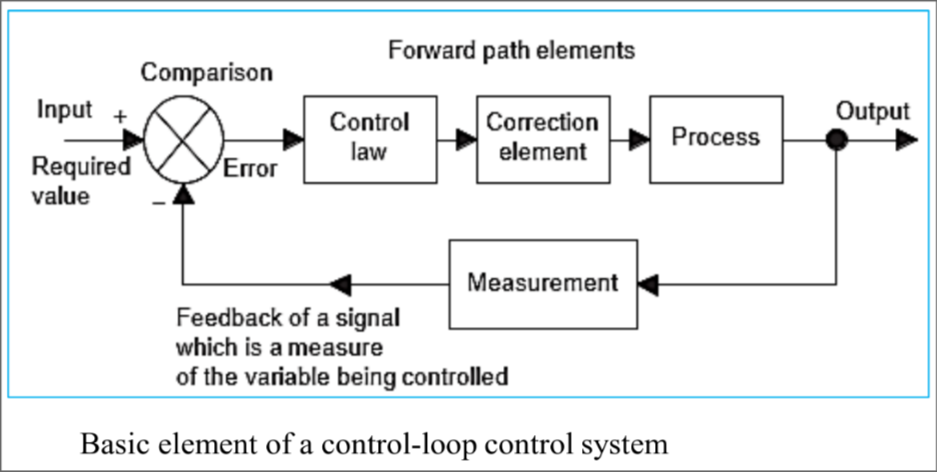
Feedback control system

Regulator system

• Maintain constant output
• Input is seldom changed

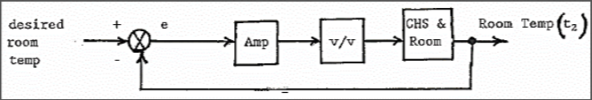
Follow-up system

• set point frequently changed

---

Application of Control Theory

Dynamic Analysis

Determination of response of a plant to commands, disturbances and changes in plant parameter

Control System Design

If dynamic analysis is unsatisfactory and modification of plant is unacceptable, design phase in necessary to select control elements needed to improve dynamic performance to acceptable level

Method of Analysis

1. Consider system performance in time domain by measuring output response for given input
2. Frequency domain - output response to sinusoidal input is considered in steady state only if transient is allowed to subside before measurement ends

Requirement of Control Theory

1. Stability
2. Accuracy - in terms of errors
   1. Error - steady state - due to static friction as output ceases to move
   2. Error - can reverse sign, overshoot due to energy
3. Speed of response

Stability and accuracy are incompatible

A good design is a compromise of both

---

Systems Classification

Stationary vs Non-stationary System

Non stationary

• differential / difference eq have one or more coefficients as functions of time

Stationary

• differential / difference eq only have constant coefficient

Linear vs non linear systems

Linear - Solution linearly related to inputs

Non-Linear - contain nonlinear terms (e.g. quadratic)

Lumped parameter vs Distributed parameter

Lumped parameter - ordinary differential equations

Distributed parameter - partial differential equations

E.g:

bodies	rigid	elastic
spring	massless	have distributed mass
electrical leads	resistanceless	distributed resistance

Continuous vs Discrete variable system

all system variables are continuous function of time	has one or more variable known only at a particular instant of time
describing equations are differential equations	equations are difference equations
	e.g. time interval controlled sampled data system

---

Laplace transforms

Let F(s) be the Laplace transform of f(t),

$$\mathcal{L}\{f\}=F(s)={\int }_0^{\infty }{e}^{-st}f(t)dt$$

Where,

$$s=\sigma +j\omega$$

Then,

$$\mathcal{L}\left\{\frac{df}{dt}\right\}=sF(s)-f(0)$$ $$\mathcal{L}\left\{\frac{d^{2}f}{d{t}^2}\right\}=s^{2}F(s)-sf(0)-\frac{df}{dt}(0)$$ $$\mathcal{L}\left\{\frac{d^{n}f}{d{t}^n}\right\}=s^{n}F(s)-\sum _{i=1}^n{s}^{n-i}\left[\frac{d^{i-1}f}{d{t}^{i-1}}\right]$$

Shift theorum

• In automatic control systems, it is known as dead time
• In the process industry, it is known as transport lag

$$\mathcal{L}\{e^{-at}f(t)\}=F(s+a)$$ $$\mathcal{L}\{f(t+a)\}=e^{as}F(s)$$

Convolution theorum

• The convolution theorum is the product of 2 Laplace transforms to form the Laplace transform of the convolution integral
• $\tau$ is known as the dummy time variable

$${\mathcal{L}}^{-1}\{X(s)Y(s)\}={\int }_0^{t}x(t-\tau )y(\tau )d\tau$$ $$={\int }_0^{t}y(t-\tau )x(\tau )d\tau$$

Final Value Theorum (for this course)

Useful in determining steady state accuracy

$$\underset{t\to \infty }{\lim }f(t)=\underset{s\to 0}{\lim }sF(s)$$

Initial Value Theorum

Useful in Inverse transform when initial condition is known to be zero

$$\underset{t\to 0^{+}}{\lim }f(t)=\underset{s\to \infty }{\lim }sF(s)$$

---

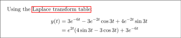
Laplace transform table

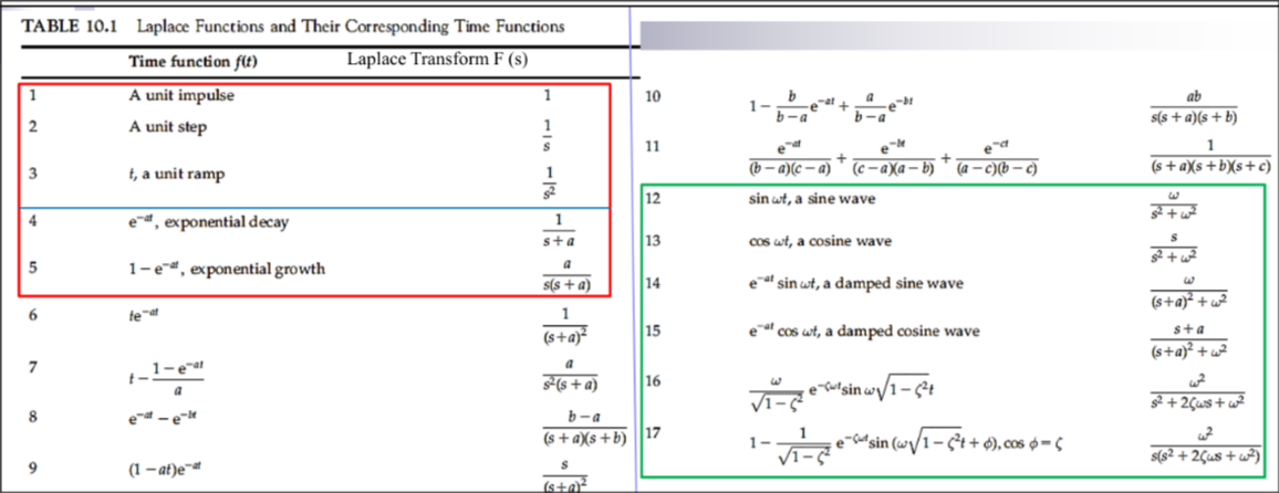
• Those in the boxes will be used
• Those in the green box is provided in the final exam

Expand for partial fraction recap!

---

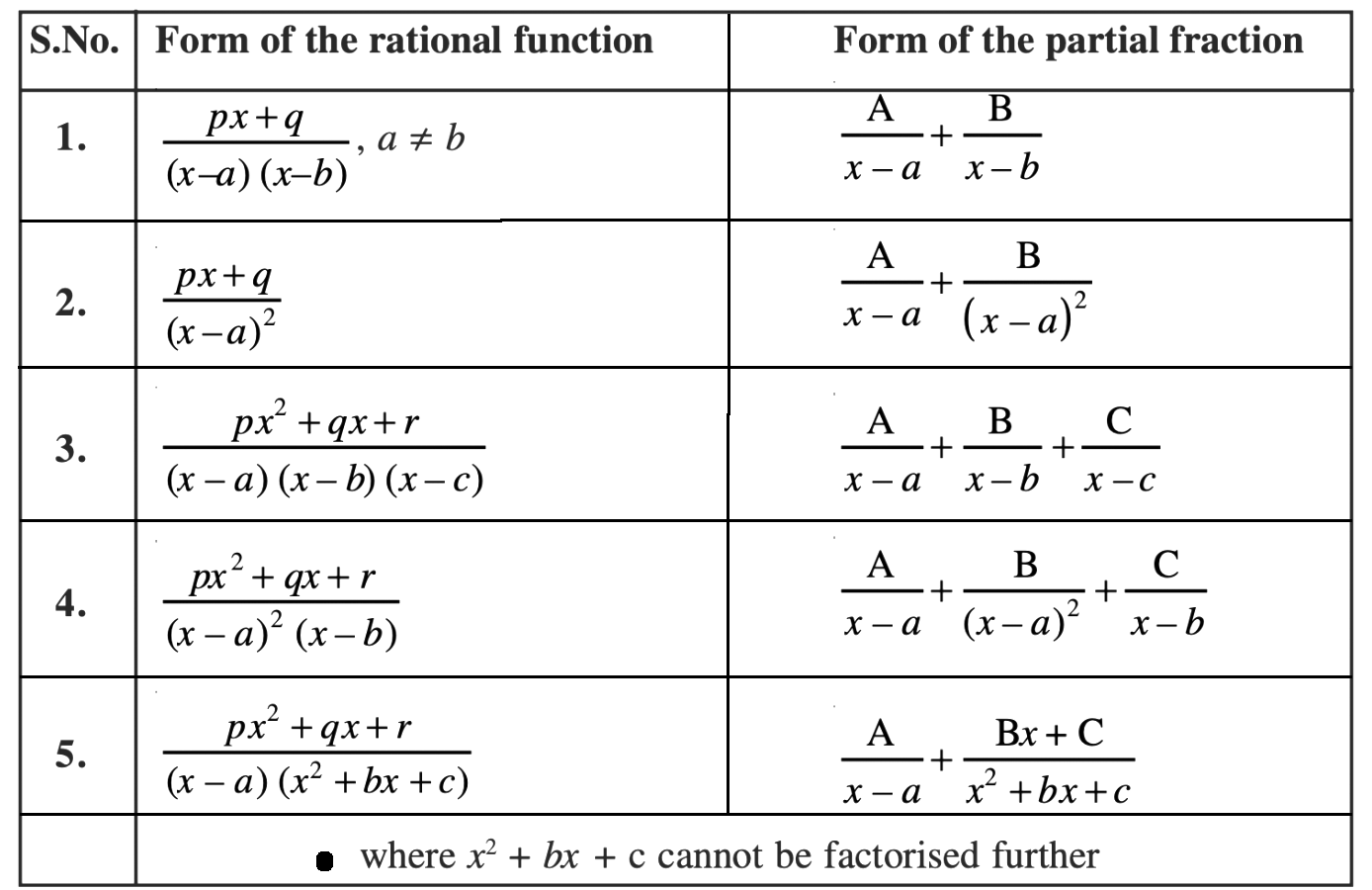
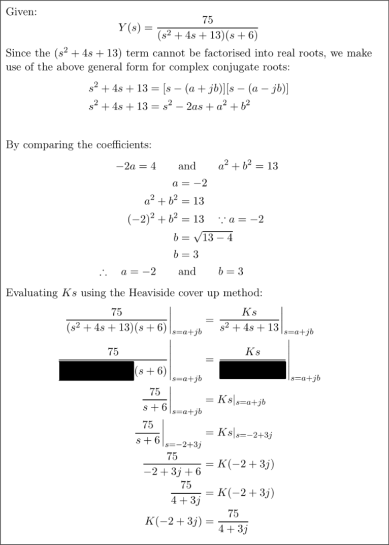
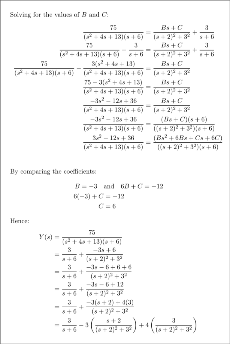
Inverse Laplace Transform for complex conjugate roots

Given a Laplace transform as a fraction:

$$\begin{array}{rl}Y(s)& =\frac{C}{[s-(a+jb)][s-(a-jb)](s-r_1)}\\ & =\frac{C}{(s^2-2as+a^2+b^2)(s-r_1)}\\ & =\frac{Ks}{s^2-2as+a^2+b^2}+\frac{K_1}{s-r_1}\end{array}$$

Where:

• $C$, $K$ and $K_1$ are constants
• $(a\pm jb)$ are the complex conjugate roots
• $(s-r_1)$ is the remaining root

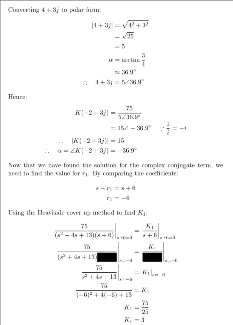
The general form of the inverse transformation for the above Laplace transformation with complex conjugate roots $(Y(s))$ is:

$$y(t)=\frac{1}{b}|K(a+jb)|e^{at}\sin (bt+\alpha )+K_1{e}^{r_{1}t}$$

Where:

• $\alpha$ is the angle from the polar form of $K(a+jb)$

The response term is just the general form without the $K_1$ term:

$$\begin{array}{rl}y(t)& =\frac{1}{b}|K(a+jb)|e^{at}\sin (bt+\alpha )\\ & =\frac{1}{b}{e}^{at}|K(a+jb)|(\cos \alpha \sin bt+\sin \alpha \cos bt)\\ & =\frac{1}{b}{e}^{at}(A\sin bt+B\cos bt)\end{array}$$

Where:

• $A=|K(a+jb)|\cos \alpha$
• $B=|K(a+jb)|\sin \alpha$

Expand this for examples!

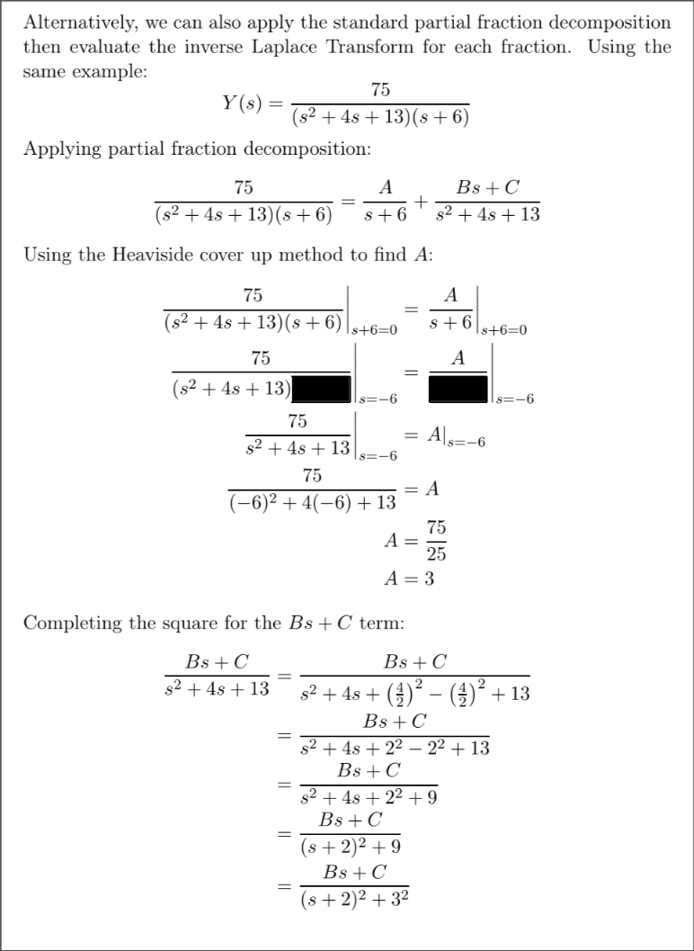
Method 1 Method 2

---

Percentage Overshoot

$\text{Percentage overshoot}=e^{-\frac{\pi \zeta }{\sqrt{1-{\zeta }^2}}}$

---

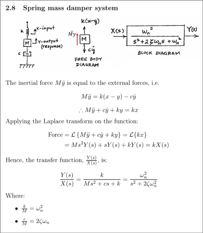
Spring damper system

sorry i got lazy here, here’s a screenshot

References